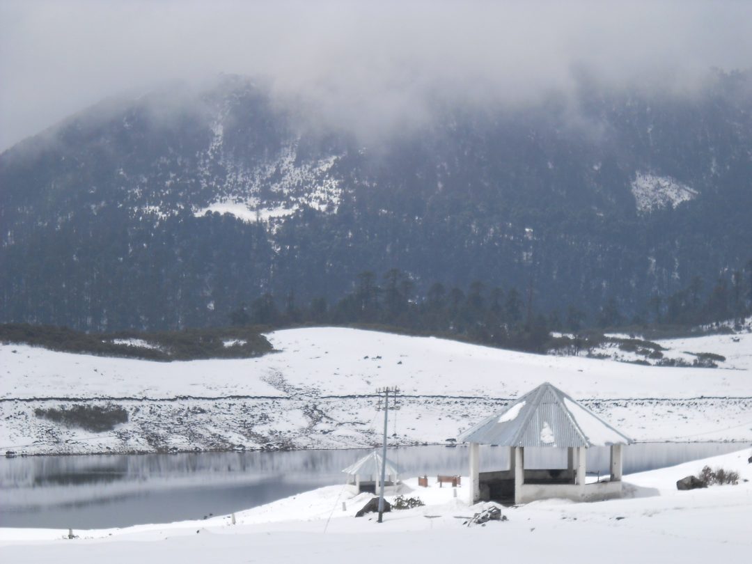
For centuries now, people living on the foothills of Bhutan have been dependent on rivers and rivulets flowing down from the mighty Himalayas. The sharing of water and other natural resources has been much dependent on the geo-political climate between the two countries.
Fortunately, the diplomatic relations between the Government of Indian and Royal Government of Bhutan have always been cordial except for localized conflicts in different border areas. Taking positive advantage of the congenial atmosphere between the two countries, NERSWN (North East Research and Social Work Networking), a Kokrajhar-based civil society organization, has been mobilizing communities on both sides of the Indo-Bhutan border along the Saralpara-Sarphang area to participate in sustainable sharing and governance of the trans-boundary river — Saralbhanga.
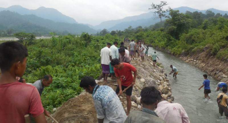
As part of the similar endeavour, more than 500 people from 36 villages of Saralpara area participated in the voluntary work to repair the traditional diversion-based irrigation system, which the locals call ‘Jamfwi/Dong’. During the ‘shramdan’ work, one of the members of the Irrigation Committee, Amarsingh Iswary said, “We are so grateful to our neighbouring country Bhutan that they have always been kind enough to allow us to draw water from Saralbhanga/Swrmanga River. This irrigation canal is the lifeline for more than 15,000 farmers in the Saralpara area alone. If the flow of water stops in this Jamfwi, we will have no option but to migrate or perish.”
The general secretary of the Irrigation Committee, Matla Mardi said, “The Saralbhanga River is the lifeline for human beings, wildlife, flora and fauna and all the living beings in Ultapani Ripu Chirang Reserve Forest. One cannot imagine life without the flow of water in this Jamfwi. We feel so fortunate that people here have become organized due to the active mobilization of NERSWN to further develop this trans-boundary irrigation system.”
The South Asian region, including India, has already started witnessing the impacts of climate change. The 2017 floods had a devastating impact in the region. India alone had a casualty of 1,046 people. Climate change-induced disasters have wider impacts and are affecting multiple countries. The ever-increasing frequency and intensity of disasters have already overwhelmed capacities of countries to respond. The regional fragilities have increased manifolds and water stress and its impact on riparian livelihoods is also an emerging problem.
There are several rivers that flow down from Bhutan to India; 56 such rivers flow down from Bhutan to Assam itself. Though these rivers are the lifeline for riparian communities in both the countries, many a time these rivers wreak havoc with flash floods, long-term inundation, erosion, cyclone and siltation. Unscientific mining, unsustainable fishing and improper water management and flood protection measures can be the determining factors for cumulative risks and vulnerabilities in the region. These rivers if governed effectively can help both the countries thrive in trade and tourism and also lead to prospering livelihood among the riparian communities.
Historically, Bhutan and India always enjoyed a friendly and cordial relationship. Both the countries exchange goods and goodwill through different established gateways called ‘Dooars’. Formal diplomatic relations between India and Bhutan were established in 1968 with the establishment of a special office of India in Thimphu. Before this, India’s relations with Bhutan were looked after by the Political Officer in Sikkim. The basic framework of India- Bhutan bilateral relations was the Treaty of Friendship and Cooperation signed in 1949 between the two countries, which was revised in February, 2007.The India-Bhutan Friendship Treaty not only reflects the contemporary nature of relationship but also lays the foundation for their future development.
The golden jubilee of the establishment of formal diplomatic relations between India and Bhutan was celebrated in the year 2018. In addition to the bilateral diplomatic relations, people-to-people ties through exchanges in the form of culture, goods and services also have been cordial between the citizens of both the countries.
Pratibha Brahma, a renowned social activist said, “Our efforts to bring together the two friendly nations for meeting the developmental aspirations of people living along the Indo-Bhutan border are bearing fruits. People-to-people ties are facilitating cordial sharing of natural resources, especially water on the border area. The Saralpara initiative for trans-border river sharing is one of the best things that I have ever seen in my life.”
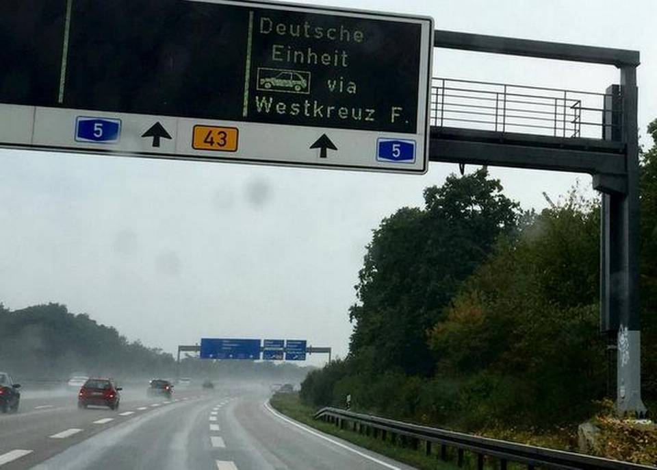
Large parts of western and central Europe sweated under blazing temperatures on June 26, with authorities in one German region imposing temporary speed limits on some stretches of the autobahn, the federal controlled-access higyway system designed for high-speed vehicular traffic, as a precaution against heat damage.
Authorities have warned that temperatures could top 40 degrees Celsius (104 Fahrenheit) in parts of the continent over the coming days as a plume of dry, hot air moves north from Africa.
The transport ministry in Germany’s eastern Saxony-Anhalt state said it has imposed speed limits of 100 kmph or 120 kmph on several short stretches of the highway until further notice. Those stretches usually have no speed limit.
On the evening of June 25, German railway operator Deutsche Bahn called rescue services to Duesseldorf Airport station as a precaution because two trains’ air conditioning systems weren’t working properly, but neither had to be evacuated.
In Paris, authorities banned older cars from the city for the day as a heat wave aggravates the city’s pollution.
Regional authorities estimate these measures affect nearly 60% of vehicles circulating in the Paris region, including many delivery trucks and older cars with higher emissions than newer models. Violators face fines.
Around France, some schools have been closed because of the high temperatures, which are expected to go up to 39 degrees Celsius (102 Fahrenheit) in the Paris area later this week and bake much of the country, from the Pyrenees in the southwest to the German border in the northeast.
Such temperatures are rare in France, where most homes and many buildings do not have air conditioning.
French charities and local officials are providing extra help for the elderly, the homeless and the sick this week, remembering that some 15,000 people, many of them elderly, died in France during a 2003 heat wave.
Prime Minister Edouard Philippe cited the heat wave as evidence of climate destabilization and vowed to step up the government’s fight against climate change.
About half of Spain’s provinces are on alert for high temperatures, which are expected to rise as the weekend approaches.
The northeastern city of Zaragoza was forecast to be the hottest on Wednesday at 39 degrees Celsius, building to 44 degrees Celsius on Saturday, according to the government weather agency AEMET.
In southwestern Europe, however, some people had other reasons to complain during their summer vacation- the Portuguese capital Lisbon, on Europe’s Atlantic coast, awoke cloudy and wet on Wednesday. AP
At Matasula village just 10 kilometres from the Ramgarh Dam, there is one hand-pump that supplies water for an entire village of 100 households.
Jaipur could run out of ground water in five years, say experts
Amid a long, harsh summer and drought in many parts of the country, Rajasthan has become one of the states where over-extraction of ground water is leading to depletion at alarming levels.
According to state government figures, in state capital Jaipur, of the 13 water blocks, 12 are in the dark zone – which means the underground water is in the danger of running out here.
“A zero water day is not very far away. Jaipur can run out of water in the next few years and cities like Ajmer and Bhilwara will probably face a zero water day even earlier,” says Dr SK Jain, a water expert and hydrologist.
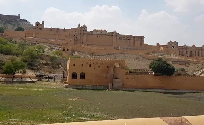
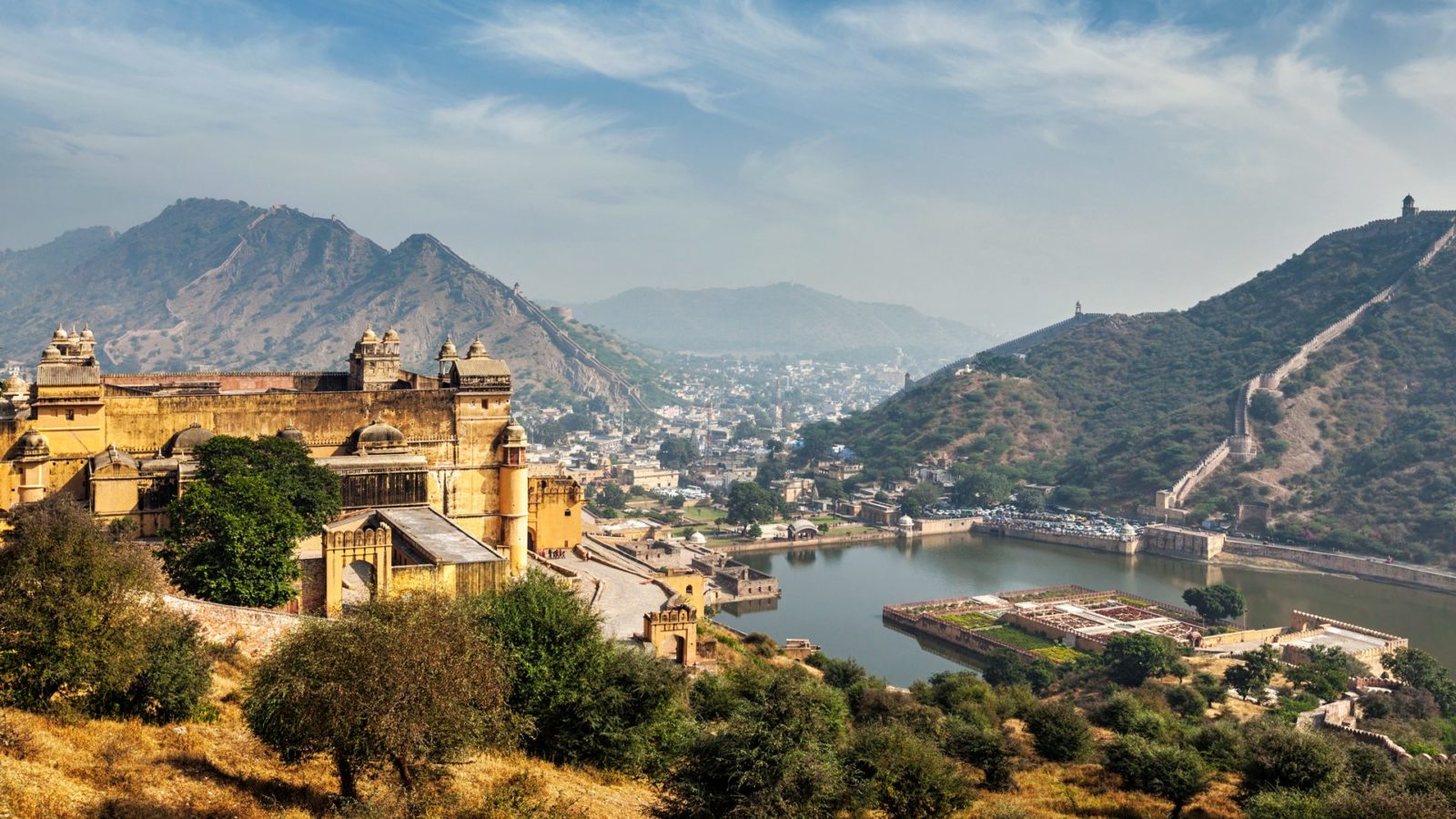
The water tanks and step well in the Amer and Jaigarh forts, ponds and tanks in villages and the Ramgarh Dam, were some of the ancient water harvesting system of medieval Jaipur that made it self-reliant in water.
The Ramgarh Dam was built in the early 1900s to supply drinking water to Jaipur city by King Madho Singh, the second. But urbanization and reckless water extraction now mean the dam is completely try and Jaipur is paying the price for its destroyed water heritage.
At Matasula village just 10 kilometres from the historic dam, there is one hand-pump that supplies water for an entire village of 100 households.
Locals recall a time not very long ago when the wells here were always brimming with water and the Ramgarh Dam contributed to ground water recharge in the area. But with the dam dry for 20 years, practically all wells in a radius of 10 kilometres have dried up too.
“When the Ramgarh Dam used to fill up during the monsoon, water used to come into our wells too. Since 2000 when the water dried up completely in the dam, our village wells have also gone dry. People have had to go for borewells as water levels have dropped,” said 40-year-old Sita Ram Jogi, a resident of Matasula village.
Women are the worst affected, says Suman, another village resident.
“We fill water all day, not only for drinking and bathing but also for our animals. Buffaloes and goats need water, and when this hand-pump stops working – sometimes it goes dry – then we have to trek many kilometres to fill water. Our children also labour with us filling water for the families daily needs,” she says.
The Rajasthan High Court has appointed a nodal officer to oversee the rejuvenation of the Ramgarh Dam.
Rohit Singh, the nodal officer in this case, says the dam has dried up due to increased agriculture, farmers building small boundaries around their fields and urbanisation in the dams catchment area, which obstructs the flow of water.
“Rajasthan has been historically water deficient but old structures like wells, stepwell tanks, we need to revive those, we need to get back to basics,” he says.COMMENT
But long term measures will not immediately resolve the water crisis in Jaipur. Every year the ground water levels in Jaipur have been dropping by 1 metre. In some blocks the extraction is 600 times more than recharge.
The U.S.-based University of California, Berkeley will adopt 100 villages in Meghalaya to start a concept of smart villages and address the issue of urban migration due to environmental issues, Chief Minister Conrad K. Sangma said on Friday. The Chief Minister was addressing a gathering at Montreux (Switzerland), who converged for the Caux Forum, which aims to inspire, equip and connect people, groups and organisations to build a just, sustainable and peaceful world.
The State government will sign the Memorandum of Understanding with the University of California, Berkeley in September to adopt 100 villages to start the concept of smart villages in Meghalaya, Mr. Conrad said, according to an official release issued here.
Our cities are already choking and having smart villages will prevent urban migration and related environmental issues, he said.
The Chief Minister spoke highly of the States’ uniqueness in terms of land ownership, forest conservation techniques as he deliberated at the Forum.
He said, “We as a government are proud of our society and the idea of our sacred groves and living root bridges should be known to the rest of the world. My government has given importance to these indigenous knowledge and have stressed on community participation in the implementation of government programmes, he said.
With a population of about 3.3 million people, the Chief Minister said the State is known worldwide for receiving the heaviest rainfall in the world.
Another great aspect of the State is the discovery by Geologists in 2018 about the Meghalayan Age which put the State in the global spotlight, he said.
Informing that about 6,500 villages are there in Meghalaya, he said the government will ensure that the National Resource Management Plans are made through full community participation.
He also informed that there is also a special emphasis on restoration of land in more than 400 villages of the State and added that the government has linked all livelihood programmes to natural resources and are encouraging people to protect these natural resources.
I am happy to inform that this year on World Environment Day we have planted 1.2 million trees and every citizen is encouraged to plant and adopt one tree, he said.
On water scarcity, the Chief Minister said Meghalaya is one of the first States in the country to be ready with the State water policy to face the issue of water conservation and water use.
There are problems we have to address and there are also solutions, we just need to come together to talk, discuss and share and need to create goals that must permeate down to the individual level so that every individual has a goal for the development and good of the society, the nation and the world, he said.
At the 2019 Dialogue at Caux, global thought leaders and practitioners will explore how community and individual actions can reverse degradation leading to peace and stability.
Himalayan glaciers supply meltwater to densely populated catchments in South Asia, and regional observations of glacier change over multiple decades are needed to understand climate drivers and assess resulting impacts on glacier-fed rivers. Here, we quantify changes in ice thickness during the intervals 1975–2000 and 2000–2016 across the Himalayas, using a set of digital elevation models derived from cold war–era spy satellite film and modern stereo satellite imagery. We observe consistent ice loss along the entire 2000-km transect for both intervals and find a doubling of the average loss rate during 2000–2016 [−0.43 ± 0.14 m w.e. year−1 (meters of water equivalent per year)] compared to 1975–2000 (−0.22 ± 0.13 m w.e. year−1). The similar magnitude and acceleration of ice loss across the Himalayas suggests a regionally coherent climate forcing, consistent with atmospheric warming and associated energy fluxes as the dominant drivers of glacier change.
INTRODUCTION
The Intergovernmental Panel on Climate Change 5th Assessment Report estimates that mass loss from glaciers contributed more to sea-level rise than the ice sheets during 1993–2010 (0.86 mm year−1 versus 0.60 mm year−1, respectively), yet uncertainties for the glacier contribution are three times greater (1). Glaciers also contribute locally to water resources in many regions and serve as hydrological buffers vital for ecology, agriculture, and hydropower, particularly in High Mountain Asia (HMA), which includes all mountain ranges surrounding the Tibetan Plateau (2, 3). Shrinking Himalayan glaciers pose challenges to societies and policy-makers regarding issues such as changing glacier melt contributions to seasonal runoff, especially in climatically drier western regions (3), and increasing risk of outburst floods due to expansion of unstable proglacial lakes (4). Yet, substantial gaps in knowledge persist regarding rates of ice loss, hydrological responses, and associated climate drivers in HMA (2).
Mountain glaciers are known to respond dynamically to a variety of drivers on different time scales, with faster response times than the large ice sheets (5, 6). In the Himalayas, in situ studies document significant interannual variability of mass balances (7–9) and relatively slower melt rates on debris-covered glacier tongues over interannual time scales (10, 11). Yet, the overall effects of surface debris cover are uncertain, as many satellite observations suggest similar ice losses relative to clean-ice glaciers over similar or longer periods (12, 13). Because of the complex monsoon climate in the Himalayas, dominant causes of recent glacier changes remain controversial, although atmospheric warming, the albedo effect due to deposition of anthropogenic black carbon (BC) on snow and ice, and precipitation changes have been suggested as important drivers (14–16).
Model projections of future Himalayan ice loss and resulting impacts require robust observations of glacier response to past and ongoing climate change. Recent satellite remote sensing studies have made substantial advances with improved spatial coverage and resolution to quantify ice mass changes during 2000–2016 (12, 17, 18), and former records extending back to the 1970s have been presented for several areas using declassified spy satellite imagery (13, 19–22). These long-term records are especially critical for extracting robust mass balance signals from the noise of interannual variability (6). Many studies also report the highly heterogeneous behavior of glaciers in localized regions, with some glaciers exhibiting faster rates of ice loss during the 21st century (20, 22). Independent analyses document simultaneously increasing atmospheric temperatures at high-elevation stations in HMA (23–26). To robustly quantify the regional sensitivity of these glaciers to climate change, a reliable Himalaya-wide record of ice loss extending back several decades is needed.
Here, we provide an internally consistent dataset of glacier mass change across the Himalayan range over approximately the past 40 years. We use recent advances in digital elevation model (DEM) extraction methods from declassified KH-9 Hexagon film (27) and ASTER stereo imagery to quantify ice loss trends for 650 of the largest glaciers during 1975–2000 and 2000–2016. All aspects of the analysis presented here only use glaciers with data available during both time intervals unless specified otherwise. We investigate glaciers along a 2000-km transect from Spiti Lahaul to Bhutan (75°E to 93°E), which includes glaciers that accumulate snow primarily during winter (western Himalayas) and during the summer monsoon (eastern Himalayas), but excludes complications of surging glaciers in the Karakoram and Kunlun regions where many glaciers appear to be anomalously stable or advancing (2). Our compilation includes glaciers comprising approximately 34% of the total glacierized area in the region, which represents roughly 55% of the total ice volume based on recent ice thickness estimates (15, 28). This diverse dataset adequately captures the statistical distribution of large (>3 km2) glaciers, thus providing the first spatially robust analysis of glacier change spanning four decades in the Himalayas. We extract DEMs from declassified KH-9 Hexagon images for the 650 glaciers, compile a corresponding set of modern ASTER DEMs, fit a robust linear regression through every 30-m pixel of the time series of elevations, sum the resulting elevation changes for each glacier, divide by the corresponding areas, and translate the volume changes to mass using a density conversion factor of 850 ± 60 kg m−3(see Materials and Methods).
RESULTS
Glacier mass changes
Our results indicate that glaciers across the Himalayas experienced significant ice loss over the past 40 years, with the average rate of ice loss twice as rapid in the 21st century compared to the end of the 20th century (Fig. 1). We calculate a regional average geodetic mass balance of −0.43 ± 0.14 m w.e. year−1 (meters of water equivalent per year) during 2000–2016, compared to −0.22 ± 0.13 m w.e. year−1 during 1975–2000 (−0.31 ± 0.13 m w.e. year−1 for the full 1975–2016 interval) (see Materials and Methods). A 30-glacier moving average shows a quasi-consistent trend across the 2000-km longitudinal transect during both time intervals (Fig. 1), and subregions have similar means and distributions of glacier mass balance. Some central catchments deviate somewhat from the Himalaya-wide mean during 2000–2016 (by approximately 0.1 to 0.2 m w.e. year−1) in the Uttarakhand (~79.0° to 80.0°E), the Gandaki catchment (~83.5° to 84.5°E), and the Karnali catchment (~81° to 83°E), which has fewer larger glaciers and relatively incomplete data coverage. Similar to previous in situ and satellite-based studies (18, 29), we observe considerable variation among individual glacier mass balances, with area-weighted SDs of 0.1 and 0.2 m w.e. year−1during each respective interval for the 650 glaciers. This variability most likely reflects different glacier characteristics such as sizes of accumulation zones relative to ablation zones, topographic shading, and amounts of debris cover. Yet, we find that, in our survey (using a rough average of 60 glaciers per 7000-km2 subregion), local variations tend to average out and mean values are similar across most catchments.
Fig. 1Map of glacier locations and geodetic mass balances for the 650 glaciers.Circle sizes are proportional to glacier areas, and colors delineate clean-ice, debris-covered, and lake-terminating categories. Insets indicate ice loss, quantified as geodetic mass balances (m w.e. year−1) plotted for individual glaciers along a longitudinal transect during 1975–2000 and 2000–2016. Both inset plots are horizontally aligned with the map view. Gray error bars are 1σ uncertainty, and the yellow trend is the (area-weighted) moving-window mean, using a window size of 30 glaciers.
Contrasting distributions of glacier mass balances are evident when comparing between time intervals. The 1975–2000 distribution has a negative tail extending to −0.6 m w.e. year−1, while the 2000–2016 distribution is more negative, extending to −1.1 m w.e. year−1 (Fig. 2A). During the more recent interval, glaciers are losing ice twice as fast on average (Fig. 2B), though this varies somewhat between subregions. For example, we find that the average rate of ice loss has increased by a factor of 3 in the Spiti Lahaul region, and by a factor of 1.4 in West Nepal. We also compile altitudinal distributions of ice thickness change for the glaciers and create a Himalaya-wide average thickness change profile versus elevation (Fig. 2, C and D). These distributed thinning profiles are a function of both thinning by mass loss and of dynamic thinning due to ice flow. We find that the 2000–2016 thinning rate (m year−1) profile is considerably steeper, which is likely caused by a combination of faster mass loss and widespread slowing of ice velocities during the 21st century (2, 30).
Fig. 2Comparison of ice losses between 1975–2000 and 2000–2016 for the 650 glaciers.(A) Histograms of individual glacier geodetic mass balances (m w.e. year−1) during 1975–2000 (mean = −0.21, SD = 0.15) and 2000–2016 (mean = −0.41, SD = 0.24). Shaded regions behind the histograms are fitted normal distributions. (B) Result of dividing the modern (2000–2016) mass balances by the historical (1975–2000) mass balances for each glacier, showing the resulting distribution of the mass balance change (ratio) between the two intervals (mean = 2.01, SD = 1.36). In this case, the shaded region is a fitted kernel distribution. (C) Altitudinal distributions of ice thickness change (m year−1) separated into 50-m elevation bins during the two intervals. (D) Normalized altitudinal distributions of ice thickness change. Normalized elevations are defined as (z − z2.5)/(z97.5 − z2.5), where z is elevation and subscripts indicate elevation percentiles. This scales all glaciers by their elevation range (i.e., after scaling, glacier termini = 0 and headwalls = 1), allowing for more consistent comparison of ice thickness changes across glaciers with different elevation ranges. Note the abrupt inflection point in the 2000–2016 profile at ~0.1; this is likely due to retreating glacier termini. Shaded regions in the altitudinal distributions indicate the SEM estimated as σz/nz−−√, where σz is the SD of the thinning rate for each 50-m elevation bin and nz is the number of independent measurements when accounting for spatial autocorrelation (see Materials and Methods).
We multiply geodetic mass balances by the full glacierized area in the Himalayas between 75° and 93° longitude to estimate region-wide ice mass changes of −7.5 ± 2.3 Gt year−1 during 2000–2016, compared to −3.9 ± 2.2 Gt year−1 during 1975–2000 (−5.2 ± 2.2 Gt year−1 during the full 1975–2016 interval). Recent models using Shuttle Radar Topography Mission (SRTM) elevation data for ice thickness inversion estimate the total glacial ice mass in our region of study to be approximately 700 Gt in the year 2000 (see Materials and Methods) (15, 28). If this estimate is accurate, our observed annual mass losses suggest that of the total ice mass present in 1975, about 87% remained in 2000 and 72% remained in 2016.
Comparison of clean-ice, debris-covered, and lake-terminating glaciers
We study mass changes for different glacier types by separating glaciers into clean-ice (<33% area covered by debris), debris-covered (≥33% area covered by debris), and lake-terminating categories based on a Landsat band ratio threshold and manual delineation of proglacial lakes (see Materials and Methods). All three categories have undergone a similar acceleration of ice loss (Table 1), and debris-covered glaciers exhibit similar and often more negative geodetic mass balances compared to clean-ice glaciers over the past 40 years (Fig. 3). Altitudinal distributions indicate slower thinning for lower-elevation regions of debris-covered glaciers (glacier tongues where debris is most concentrated) relative to clean-ice glaciers, but comparatively faster thinning in mid- to upper elevations (Fig. 4). Lake-terminating glaciers concentrated in the eastern Himalayas exhibit the most negative mass balances due to thermal undercutting and calving (31), though they only comprise around 5 to 6% of the estimated total Himalaya-wide mass loss during both intervals.Table 1Himalaya-wide geodetic mass balances (m w.e. year−1).View this table:
Fig. 3Comparison between clean-ice (<33% debris-covered area) and debris-covered (≥33% debris-covered area) glaciers for seven subregions.Circle sizes are proportional to glacier areas, colors delineate clean-ice versus debris-covered categories, and boxplots indicate geodetic mass balance (m w.e. year−1). Box center marks (red lines) are medians; box bottom and top edges indicate the 25th and 75th percentiles, respectively; whiskers indicate q75 + 1.5 ⋅ (q75 − q25) and q25 − 1.5 ⋅ (q75 − q25), where subscripts indicate percentiles and “+” symbols are outliers.Fig. 4Altitudinal distributions of ice thickness change (m year−1) for the 650 glaciers.Glaciers are separated by time interval (top) and category (<33% versus ≥33% debris-covered area) (bottom). (A) Altitudinal distributions of ice thickness change for clean-ice glaciers during 1975–2000 and 2000–2016. The y axes are normalized elevation as in Fig. 2. (B) Same as (A), but for debris-covered glaciers. (C) Altitudinal distributions of ice thickness change during 1975–2000 for clean-ice and debris-covered glaciers. (D) Same as (C), but for 2000–2016. (E) Altitudinal distributions of glacierized area for both glacier categories. Elevational extent of debris cover varies widely between individual glaciers, but is mostly concentrated in lower ablation zones. The clean-ice category includes 478 glaciers and the debris-covered category includes 124 glaciers.
Approximation of required temperature change
As a first approximation of the consistency between observed glacier mass balances and available temperature records, we estimate the energy required to melt the observed ice losses and conservatively estimate the atmospheric temperature change that would supply this energy via longwave radiation to the glaciers, using a simple energy balance approach (Materials and Methods). We propagate significant uncertainties associated with input from global climate reanalysis data, scaling of temperatures from coarse reanalysis grids to specific glacier elevations, and averaging of climate data over the glacierized region. Results suggest that the observed acceleration of ice loss can be explained by an average temperature ranging from 0.4° to 1.4°C warmer during 2000–2016, relative to the 1975–2000 average. This approximately agrees with the magnitude of warming observed by meteorological stations located throughout HMA, which have recorded air temperatures around 1°C warmer on average during 2000–2016, relative to 1975–2000 (Fig. 5). More comprehensive climate observations and models will be essential for further investigation, but these simple energy constraints suggest that the acceleration of mass loss in the Himalayas is consistent with warming temperatures recorded by meteorological stations in the region.
Fig. 5Compilation of previously published instrumental temperature records in HMA.(A) Regional temperature anomalies, relative to the 1980–2009 mean temperatures for each record. The yellow trend (23) from the quality-controlled and homogenized climate datasets LSAT-V1.1 and CGP1.0 recently developed by the China Meteorological Administration (CMA), using approximately 94 meteorological stations located throughout the Hindu Kush Himalayan region. The orange trend (44) is from a similar CMA dataset derived from 81 stations more concentrated on the eastern Tibetan Plateau. The blue trend (24) is from three decades of temperature data from 13 mountain stations located on the southern slopes of the central Himalayas. The black trend is the 5-year moving mean. (B) Temperature anomalies from high-elevation stations at the Chhota Shigri glacier terminus (25); Dingri station in the Everest region (26); average from the Kanzalwan, Drass, and Patseo stations (45); and average of 16 stations above 4000 m elevation on the Tibetan Plateau and eastern Himalayas (46). Here, temperature anomalies are relative to the mean of each record. The gray trend line is the 5-year moving mean. (C) Difference in mean temperature (°C) between the two intervals, i.e., the mean of the 2000–2016 interval relative to the mean of the 1975–2000 interval.
DISCUSSION
Implications for dominant drivers of glacier change in the Himalayas
The parsing of Himalayan glacier energy budgets is not a straightforward task owing to the scarcity of meteorological data, in combination with the complex climate and topography of the region (2). Furthermore, the Himalayas border hot spots of high anthropogenic BC emissions, which may affect glaciers by direct heating of the atmosphere and decreasing albedo of ice and snow after deposition (14). While improved analyses combining observations and high-resolution atmospheric and glacier energy balance models will be required to quantify these effects, the pattern of ice loss we observe has important implications regarding dominant climate influences on Himalayan glacier mass balances. Our results suggest that any drivers of glacier change must explain the region-wide consistency, the doubling of the average rate of ice loss in the 21st century compared to 1975–2000, and the observation that clean-ice, debris-covered, and lake-terminating glaciers have all experienced a similar acceleration of mass loss.
Some studies have suggested a weakening of the summer monsoon and reduced precipitation as primary reasons for negative glacier mass balances, particularly in the Everest region (16). While decreasing accumulation rates may account for a significant portion of the mass balance signal for some glaciers, an extreme Himalaya-wide decrease in precipitation would be required to explain the extensive ice losses we observe, especially given that monsoon-dominated glaciers with high accumulation rates are known to be much more sensitive to temperature than accumulation changes (5, 32). Regional studies of precipitation trends in the Himalayas do not suggest a widespread decrease in precipitation over the past four decades (Supplementary Materials). A uniform BC albedo forcing across the Himalayas is another possible explanation, although BC concentrations measured in snow and ice in the Himalayas have been found to be spatially heterogeneous (14, 33), and high-resolution atmospheric models also show large spatial variability of deposited BC originating from localized emissions in regions of complex terrain (14, 34). Future analyses focused on quantifying the spatial patterns of BC deposition will reveal further insights, yet given the rather homogeneous pattern of mass loss we observe across the 2000-km Himalayan transect, a strong, spatially heterogeneous mechanism seems improbable as a dominant driver of glacier ice loss in the region.
Debris-covered glaciers
Similar thinning rates of debris-covered (thermally insulated) glaciers relative to clean-ice glaciers have been observed by previous studies and have been not only ascribed to surface melt ponds and associated ice cliffs acting as localized hot spots to concentrate melting but also attributed to declining ice flux causing dynamic thinning and stagnation of debris-covered glacier tongues (2). While we cannot yet directly deconvolve relative contributions from these processes, we find that average thinning rates for debris-covered glaciers are slower than clean-ice glaciers at low elevations (glacier tongues where debris is most concentrated), which agrees with reduced melt rates from field studies. In turn, debris-covered glaciers tend to have comparatively faster thinning at mid-range elevations, where debris cover is sparser and also where the majority of total glacierized area resides (Fig. 4). Models of debris-covered glacier processes suggest that this pattern of thinning may cause a reduction in down-glacier surface gradient, which, in turn, reduces driving stress and ice flux and explains why debris-covered ablation zones become stagnant (35). We also find that clean-ice glaciers exhibit a much more pronounced steepening of the thinning profile over time, compared to debris-covered glaciers. It may be that both glacier types experience a uniform thinning phase followed by a changing terminus flux and retreat phase, but the clean-ice glaciers are in a later phase of response to recent climate change (36).
Comparison with previous studies in the Himalayas
To compare our results with previous remote sensing studies that derive mass changes from various sensors (including Hexagon, SRTM, SPOT5, ICESat, and ASTER), we restrict our results to the approximate geographical regions covered by each corresponding study (12, 13, 17–22) and then compute area-weighted average geodetic mass balances. In addition, we compare individual glacier mass balances for the Everest and Langtang Himal regions, where mass changes were previously estimated using declassified Corona and Hexagon imagery (13, 19, 20). Despite factors such as variable spatial resolutions, distinct void-filling methods, heterogeneous spatial and temporal coverages, and different definitions of glacier boundaries, we find that our average mass balances generally agree with previous analyses and overlap within uncertainties (table S1). However, because of the significant variability of individual glacier mass changes within subregions, our results also highlight the importance of sampling a large number of glaciers to obtain a robust average trend for any given area.
Comparison with benchmark mid-latitude glaciers and global average
To gain perspective on mass losses from these low-latitude glaciers in the monsoonal Himalayas, we compare our results with benchmark mid-latitude glaciers in the European Alps, as well as with a global average mass balance trend (fig. S1) (37). The Alps contain the most detailed long-term glaciological and high-elevation meteorological records on Earth, and the climatic sensitivity and behavior of these European glaciers are well understood compared to glaciers in HMA. Air temperatures in the Alps show an abrupt warming trend beginning in the mid-1980s, and Alpine mass balance records display a concurrent acceleration of ice loss, with a continual strongly negative mass balance after that time. Himalayan weather station data indicate a more gradual warming trend, with the strongest warming beginning in the mid-1990s (fig. S1, A and B). We find that mass balance in the Himalayas is less negative compared to the Alps and the global average, despite close proximity to a known hot spot of increasing BC emissions with rapid growth and accompanying combustion of fossil fuels and biomass in South Asia (38). The concurrent acceleration of ice loss observed in both the Himalayas and Europe over the past 40 years coincides with a distinct warming trend beginning in the latter part of the 20th century, followed by the consistently warmest temperatures through the 21st century in both regions.
Conclusion
Our analysis robustly quantifies four decades of ice loss for 650 of the largest glaciers across a 2000-km transect in the Himalayas. We find similar mass loss rates across subregions and a doubling of the average rate of loss during 2000–2016 relative to the 1975–2000 interval. This is consistent with the available multidecade weather station records scattered throughout HMA, which indicate quasi-steady mean annual air temperatures through the 1960s to the 1980s with a prominent warming trend beginning in the mid-1990s and continuing into the 21st century (23–26). We suggest that degree-day and energy balance models focused on accurately quantifying glacier responses to air temperature changes (including energy fluxes and associated feedbacks) will provide the most robust estimates of glacier response to future climate scenarios in the Himalayas.
MATERIALS AND METHODS
Hexagon
U.S. intelligence agencies used KH-9 Hexagon military satellites for reconnaissance from 1973 to 1980. A telescopic camera system acquired thousands of photographs worldwide, after which film recovery capsules were ejected from the satellites and parachuted back to Earth over the Pacific Ocean. With a ground resolution ranging from 6 to 9 m, single scenes from the mapping camera cover an area of approximately 30,000 km2 with overlap of 55 to 70%, allowing for stereo photogrammetric processing of large regions. Images were scanned by the U.S. Geological Survey (USGS) at a resolution of 7 μm and downloaded via the Earth Explorer user interface (earthexplorer.usgs.gov). Digital elevation models were extracted using the Hexagon Imagery Automated Pipeline methodology, which is coded in MATLAB and uses the OpenCV library for Oriented FAST and Rotated BRIEF (ORB) feature matching, uncalibrated stereo rectification, and semiglobal block matching algorithms (27). The majority of the KH-9 images here were acquired within a 3-year interval (1973–1976), and we processed a total of 42 images to provide sufficient spatial coverage (fig. S2).
ASTER
The ASTER instrument was launched as part of a cooperative effort between NASA and Japan’s Ministry of Economy, Trade and Industry in 1999. Its nadir and backward-viewing telescopes provide stereoscopic capability at 15-m ground resolution, and a single DEM covers approximately 3600 km2. Approximately 26,000 ASTER DEMs were downloaded via the METI AIST Data Archive System (MADAS) satellite data retrieval system (gbank.gsj.jp/madas), a portal maintained by the Japanese National Institute of Advanced Industrial Science and Technology and the Geological Survey of Japan. To use all cloud-free pixels (including images with a high percentage of cloud cover), no cloud selection criteria were applied when downloading the images. We used the Data1.l3a.demzs geotiff product, which has a spatial resolution of 30 m. After downloading, the DEMs were subjected to a cleanup process: For a given scene, any saturated pixels (i.e., equal to 0 or 255) in the nadir band 3 (0.76 to 0.86 μm) image were masked in the DEM. Next, the SRTM dataset was used to remove any DEM values with an absolute elevation difference larger than 150 m (relative to SRTM), which effectively eliminated the majority of errors caused by clouds. While more sophisticated cloud masking procedures are possible, the ASTER shortwave infrared detectors failed in April 2008, making cloud detection after this time impossible using standard methods. We examined existing cloud masks derived using Moderate Resolution Imaging Spectroradiometer images as another option (tonolab.cis.ibaraki.ac.jp/ASTER/cloud/). However, these are not optimized for snow-covered regions and often misclassify glacier pixels as clouds. Instead, our large collection of multitemporal ASTER scenes, the SRTM difference threshold, and our robust linear trend fitting algorithm [see description of Random Sample Consensus (RANSAC) in the “Trend fitting of multitemporal DEM stacks” section] effectively excluded any remaining erroneous cloud elevations after the initial threshold. As a final step, all ASTER DEMs were coregistered to the SRTM using a standard elevation–aspect optimization procedure (39). We did not apply fifth-order polynomial correction procedures to the ASTER DEMs for satellite “jitter” effects and curvature bias as done in some previous studies (18). We found that while these types of corrections may reduce the overall average elevation error in a scene, the polynomial fitting can be unwieldy and may introduce unwanted localized biases. By stacking many ASTER DEMs (with 20.5 being the average number of observations per pixel stack during the ASTER trend fitting, see fig. S3E) and using a robust fitting procedure, we found that biases do not correlate across overlapping scenes, and thus tend to cancel out one another. Furthermore, the elevation change results from this portion of our study overlap within uncertainties with Brun et al. (18) (Supplementary Materials) who did perform polynomial corrections. This suggests that for a large-scale regional study using a high number of overlapping ASTER scenes, the satellite jitter and curvature bias corrections have a relatively minimal impact on the final results.
Glacier polygons
To delineate glaciers during all portions of the analysis, we used manually refined versions of the Randolph Glacier Inventory (RGI 5.0) (40). Starting with the original RGI dataset, we edited the glacier polygons to reflect glacier areas during 1975, 2000, and 2016. For the 1975 edit, we used a combination of Hexagon imagery, the Global Land Survey (GLS) Landsat Multispectral Scanner mosaic (GLS1975), and glacier thickness change maps derived from differencing the Hexagon and modern ASTER DEMs, which are particularly useful for debris-covered glacier termini that often have spectral characteristics indistinguishable from surrounding terrain. Debris-covered areas for each glacier were delineated using a Landsat DN TM4/TM5 band ratio with a threshold of 2.0, and glaciers with ≥33% debris cover were assigned to the debris-covered category. For the 2000 edit, we used the GLS2000 Landsat Enhanced Thematic Mapper Plus mosaic, along with glacier thickness change maps derived from differencing ASTER DEMs. For the 2016 edit, we used a custom mosaic of Landsat 8 imagery with acquisition dates spanning 2014–2016. The individually edited glacier polygons were used for all ice volume change and geodetic mass balance computations. The polygons were also used during alignment of the DEMs, where the shapefiles were converted to raster masks with a dilation (morphological operation) of 250 m on the binary rasters. This effectively excluded unstable terrain surrounding the glaciers during the DEM alignment process, such as steep avalanching slopes and unstable moraines.
Trend fitting of multitemporal DEM stacks
Glacier polygons were processed individually—all DEMs from a given time interval (1975–2000 or 2000–2016) that overlap a polygon were selected and resampled to the same 30-m resolution using linear interpolation. The overlapping DEMs were sampled with a 25% extension around each glacier to include nearby stable terrain for alignment and uncertainty analysis (fig. S4). After ensuring that there is no vertical bias, the aligned DEMs were sorted in temporal order as a three-dimensional matrix, and linear trends were fit to every pixel “stack” (i.e., along the third dimension of the matrix) using the RANSAC method. During each RANSAC iteration, a random set of two elevation pixels per stack were selected. A linear trend was fit to these two values, and then all remaining elevation pixels were compared to the trend. Any elevation pixels within 15 m of the trend line were marked as inliers. This process was repeated for 100 iterations, and the iteration with the greatest number of inliers was selected. A final linear fit was performed using all inliers from the best iteration, and this trend was used for each pixel stack’s thickness change estimate. The thickness change maps were subjected to outlier removal using thresholds for maximum slope, maximum thickness change, minimum count per pixel stack, minimum timespan per pixel stack, maximum SD of inlier elevations per pixel stack, and maximum gradient of the thickness change map (fig. S3). In addition, the thickness change pixels were separated into 50-m elevation bins, and pixels falling outside the 2 to 98% quantile range were excluded. Any bins with less than 100 pixels were removed and then interpolated using the two adjacent bins. Before computing ice volume change for the glaciers, the final thickness change maps were visually inspected, any remaining erroneous pixels (which occurred almost exclusively in low-contrast, snow-covered accumulation zones) were manually masked, and a 5 × 5 pixel median filter was applied. We did not attempt to perform seasonality corrections, as no seasonal snowfall records are available and because nearly all the Hexagon DEMs were acquired during winter, thus minimizing any seasonality offsets between regions. For the 1975–2000 interval, we used the Hexagon DEMs and sampled ASTER thickness change trends at the start of the year 2000. For regions with multiple overlapping Hexagon DEMs, we used the same RANSAC method. During the 1975–2000 interval, only two DEMs were available for most glaciers. In these cases, the RANSAC iterations were unnecessary, and we simply differenced the two available DEMs. We did not use SRTM for any thickness change estimates; thus, no correction for radar penetration was necessary.
Mass changes
To compute (mean annual) ice volume changes for individual glaciers, all thickness change pixels falling within a glacier polygon were transformed to an appropriate projected WGS84 UTM coordinate system (zones 43 to 46, depending on longitude of the glacier). Pixel values (m year−1) were then multiplied by their corresponding areas (pixel width × pixel height) and summed together. The resulting ice volume change was then divided by the average glacier area to obtain a glacier thickness change. We used the average of the initial and final glacier areas for a given time interval and excluded slopes greater than 45° to remove any cliffs and nunataks. Last, the glacier thickness change was multiplied by an average ice-firn density (41) of 850 kg m−3 and then divided by the density of water (1000 kg m−3) to compute glacier geodetic mass balance in m w.e. year−1. Because of cloud cover, shadows, and low radiometric contrast, some glacier accumulation zones had gaps in the DEMs and resulting thickness change maps. This is particularly evident in the Hexagon DEMs for the Spiti Lahaul region owing to extensive cloud cover. To fill these gaps, we tested two different void-filling methods for comparison. In the first method, we defined a circular search area with a radius of 50 km around the center of a given glacier. All thickness change pixels from glaciers in this surrounding area were binned (into 50-m elevation bins, and following the same outlier-removal procedure given in the preceding section), and any missing data in the glacier were set to this “regional bin” mean value at the corresponding elevation. In the second method, we filled data gaps using an interpolation procedure, where voids in an individual glacier were linearly interpolated using bin values at upper and lower elevations relative to the missing data (those belonging to the same glacier), and assumed zero change at the highest elevation bin (headwall). Both methods yielded similar results (table S1). In addition, no obvious trends were apparent when geodetic mass balance was plotted versus percent data coverage or glacier size (fig. S5). While smaller glaciers exhibited more scatter, the average mass balance was similar for all glacier sizes. These observations indicate that our representative sample of glaciers, while biased toward larger glaciers, adequately captures the statistical distribution of glacier mass balances in the Himalayas.
To calculate regional geodetic mass balances, we separated glaciers into four subregions (Spiti Lahaul, West Nepal, East Nepal, and Bhutan) as defined by Brun et al. (18). We then calculated the average mass balance for each of these four subregions, weighted by individual glacier areas. Last, we calculated a final average mass balance for the Himalayas, weighted by the total glacierized area (from the RGI 5.0 database) in each of the four subregions, between 75° to 93° longitude. Because of the relatively homogeneous mass balance distribution, we found that this approach resulted in similar values (well within the uncertainties) compared to simply calculating the area-weighted average mass balance of the 650 measured glaciers. To obtain the total mass changes in Gt year−1, we multiplied each subregion mass balance by its total glacierized area and then summed the results from all subregions to get Himalaya-wide totals of −3.9 Gt year−1 for 1975–2000 and −7.5 Gt year−1 for 2000–2016. To calculate contributions to sea-level rise, we used a global ocean surface area of 361.9 × 10⁶ km2 (fig. S4G).
To estimate the total ice mass present in our region of study, we used ice thickness estimates from Kraaijenbrink et al. (15), who used the Glacier bed Topography version 2 model to invert for ice thickness (28) with input from the SRTM DEM (acquired in February of 2000). The ice thickness estimates from (15) did not include glaciers smaller than 0.4 km2, and to estimate the additional mass contribution from these smallest glaciers (along with any other glaciers that are missing thickness estimates), we fit a second-order polynomial to the logarithm of glacier volumes versus the logarithm of glacier areas and evaluated this fit equation for any glaciers without volume data (fig. S6). We then converted glacier volume to mass using a density value of 850 kg m−3. Over our region of study, the ice volumes from the thickness data amounted to 649 Gt, with an additional contribution of 35 Gt from the fitting procedure, for a total of 684 Gt.
Uncertainty assessment
We quantified statistical uncertainty for individual glaciers using an iterative random sampling approach. For a given glacier, the SD of elevation changes from the surrounding stable terrain (σz) was first calculated. For any missing thickness change pixels within the glacier polygon, we also included an extrapolation uncertainty σe. This accounts for additional error in regions with incomplete data, i.e., those glacier regions filled by extrapolating thickness changes from surrounding glaciers, or linear interpolation assuming zero change at the headwall, as described in the previous section. We found that in the Himalaya-wide altitudinal distributions, the maximum SD of thickness change in any 50-m elevation bin above 5000 m is 0.56 m year−1. Nearly all regions with incomplete data coverage are above this elevation, resulting from poor radiometric contrast for snow-covered glacier accumulation zones. We thus conservatively set σe equal to 0.6 m year−1. We then combined both sources of error to get σp for every individual thickness change pixelσp=σ2z+σ2e−−−−−−√(1)
To account for spatial autocorrelation, we started with a normally distributed random error field (with a mean of 0 and an SD of 1) the same size as the thickness change map and then filtered it using an n-by-n moving window average to add spatial correlation, where n is defined as the spatial correlation range divided by the spatial resolution of the thickness change map. We used 500 m for the spatial correlation range, which is a conservative value based on semivariogram analysis in mountainous regions from previous studies (18, 21, 42). The resulting artificial error field En (now with spatial correlation) is scaled by the σp values and added to the thickness change map ΔH as follows, where (x, y) are pixel coordinatesΔHE(x,y)=ΔH(x,y)+En(x,y)⋅σp(x,y)σn(2)
If thickness change data exist at a given pixel location (x, y) on the glacier, σn is the SD of the set of all En values where data exist (i.e., where σe is equal to zero). Conversely, if thickness change data do not exist at a given pixel location (x, y) on the glacier, σn is the SD of the set of all En values where data do not exist (i.e., where σe is equal to 0.6 m year−1). In this way, the second term of Eq. 2 assigns larger uncertainties to regions with incomplete data. Last, all glacier thickness change pixels in ΔHE were summed together to compute a volume change with the introduced error. This procedure was repeated for 100 iterations, and the volume change uncertainty σΔV was computed as the SD of the resulting distribution (fig. S4). For region-wide volume change estimates, we conservatively assumed total correlation between glaciers and computed region-wide uncertainty as follows, where g is the total number of glaciers (~17,400)σΔV region=∑1gσΔV(3)
For glaciers where thickness change data are not available, a measure of uncertainty is still required to factor into the final regional uncertainty estimate. For these glaciers, we estimated σΔVas (42)σΔV=σ2z region⋅Acor5⋅A−−−−−−−−−−−√(4)Acor=π⋅L2(5)
In this case, σz region is the region-wide SD of elevation change over stable terrain (0.42 m year−1) (fig. S7), Acor is the correlation area, L is the correlation range (500 m), and A is the glacier area. Last, all σΔV and σΔV regjon estimates were combined with an area uncertainty (43) of 10% and a density uncertainty (41) of 60 kg m−3 using standard uncorrelated error propagation.
Sensitivity of region-wide glacier mass change estimates
We further tested the sensitivity of our region-wide estimates to potential biases, including (i) the exclusion of small glaciers, (ii) incomplete data coverage for many glacier accumulation zones during 1975–2000, and (iii) void-filling technique. First, we note that our geodetic mass balance analysis only includes glaciers larger than 3 km2. This is because mass balance uncertainties increase with decreasing glacier size, and we find that uncertainties often exceed the magnitude of mass changes for glaciers smaller than ~3 km2. To test whether the neglected small glaciers appreciably affect the result, we also computed mass balances using all available glaciers (i.e., all glaciers with ≥33% data coverage, including those smaller than 3 km2). We find that including the full set of smaller glaciers changes the region-wide geodetic mass balance estimates by a maximum of 0.04 m w.e. year−1 (fig. S4G). Next, we note that the Hexagon DEMs in particular have poor data coverage over glacier accumulation zones (figs. S8 and S9). However, the vast majority of thinning occurs in glacier ablation zones, and the amount of thinning decreases with elevation in a quasi-linear fashion, especially in mid- to upper regions of the glaciers where data gaps are most common. Thus, we hypothesize that we can extrapolate and interpolate with reasonable confidence over accumulation areas. To test the robustness of this assumption, we used the 2000–2016 glacier change data. The ASTER data over this interval have superior radiometric contrast and adequately capture elevation change trends for most accumulation zones. We first set all 2000–2016 thickness change pixels to be empty where the 1975–2000 data are missing to simulate the same data gaps over accumulation zones as in the 1975–2000 data. We then performed the same geodetic mass balance calculations and found that the region-wide geodetic mass balance only changes by 0.01 m w.e. year−1 (fig. S4G, comparing test 3 to test 1). Last, we performed two separate void-filling methods for all tests (see the “Mass changes” section for descriptions of void-filling methods) and observed a maximum change in geodetic mass balance of 0.04 m w.e. year−1. Overall, the relatively small impact of each test suggests that our results are robust to the exclusion of small glaciers, incomplete data coverage over glacier accumulation zones, and void-filling technique.
Fig. S1. Comparison of Himalayan temperature trends and regional mass balance with benchmark mid-latitude glaciers and a global average trend.
Fig. S2. Coverage of glacierized area in the Himalayas.
Fig. S3. Trend fit examples for two large glaciers using ASTER DEMs during 2000–2016, histograms of ASTER pixel counts and timespans per stack (glacier averages), and outlier thresholds.
Fig. S4. Illustration of uncertainty estimation procedure for a single iteration/glacier and Himalaya-wide sensitivity tests.
Fig. S5. Geodetic mass balances during 1975–2000 and 2000–2016 plotted against various parameters.
Fig. S6. Log-log plot of glacier volumes versus areas used to estimate the total ice mass present in our region of study.
Fig. S7. Analysis of elevation change for nonglacier pixels (stable terrain) during both intervals.
Fig. S8. Thickness change maps used in the analysis.
Fig. S9. Thickness change maps for the three remaining Himalayan regions.
Table S1. Geodetic mass balance comparisons with prior studies.
This is an open-access article distributed under the terms of the Creative Commons Attribution-NonCommercial license, which permits use, distribution, and reproduction in any medium, so long as the resultant use is not for commercial advantage and provided the original work is properly cited.
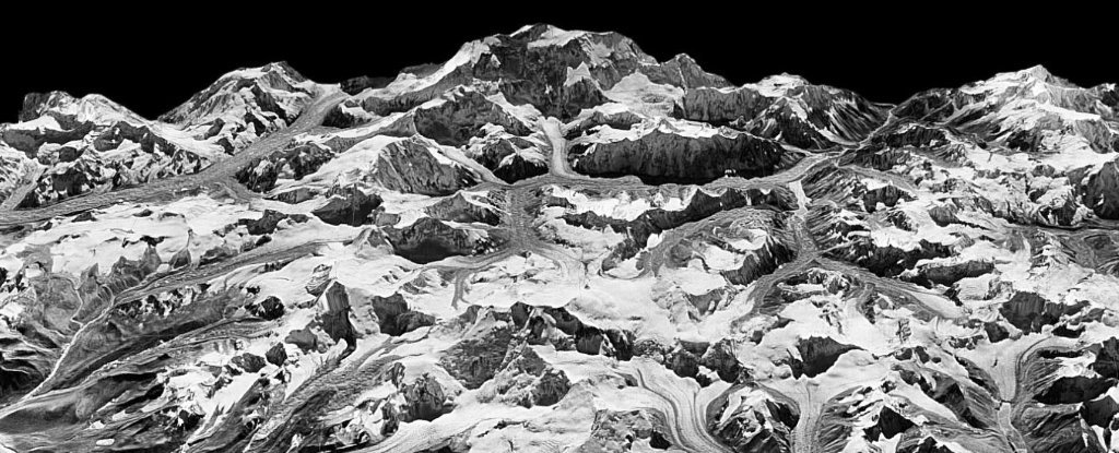
MIKE MCRAE Just under half a century ago a system of satellites codenamed Hexagon was circling the globe and snapping high-resolution shots of the changing landscape… not to mention a Russian airfield or two.
With the Cold War long melted, those images were declassified back in 2002, providing rich pickings for all kinds of research. Now scientists have used these pictures to present a startling new perspective on the Himalaya’s vanishing glaciers.
A team of US researchers from Columbia University and the University of Utah have made detailed measurements on changes to the thickness of ice in the Himalayas between two time periods; from 1975 to 2000, and then 2000 to 2016.
In some ways, what they found might not come as a great shock, if you’ve been paying attention to the climate crisis.
“It looks just like what we would expect if warming were the dominant driver of ice loss,” says the study’s lead author Joshua Maurer from Columbia University’s Lamont-Doherty Earth Observatory.
The team stitched together galleries of images of the Himalayas taken by the Keyhole-9 ‘Hexagon’ photographic reconnaissance satellites, ending up with an overview of some 650 glaciers spanning the famous mountain range.
They then developed a process to turn the 3D map into a form that provided information on elevations.
By comparing the results with modern stereo satellite imagery from NASA’s Advanced Spaceborne Thermal Emission and Reflection Radiometer (ASTER) program, Maurer and his team could calculate annual changes to ice coverage.
Since the turn of the millennium, glaciers have thinned by an average of just under half a metre (roughly 1.5 feet) per year. Over the preceding decades, that loss was half; closer to 22 centimetres, or just under 10 inches.
That’s averaged out as well. While some glaciers at higher elevations are holding steady, there are rivers of ice closer to sea level that are losing on average 5 metres (16 feet) a year.
Of course, glaciers can thin out over time for a number of reasons. Lower precipitation, for example, or fine particulates from pollution increasing localised warming by darkening the ice and absorbing sunlight.
These factors can almost certainly contribute to the melting of large patches here and there, but the sheer scale of the change implies a more global effect.
To test their suspicions, the team also compiled data on temperatures taken by ground stations and compared these with rates of melting across the map.
Sure enough, both sets of figures lined up neatly enough to reveal that our warming planet can certainly account for the ice loss.
“This is the clearest picture yet of how fast Himalayan glaciers are melting over this time interval, and why,” says Maurer.
Further west, mountain ranges such as the Alps have attracted attention for accelerated melting of their icy peaks in the 1980s.
While it took a little longer to come up to speed, it’s now clear the Himalayas are rocketing ahead. Given the area they cover and their position, we can expect the melting of their glaciers to be a catastrophe of immense proportions.
Seasonal snowmelts contribute significant quantities of water to major river systems such as the Indus, where hundreds of millions rely on its flow and volume for drinking water, farming, and hydroelectricity.
Increased melting might temporarily be a boon, but in the long term, millions of people will face an increasing risk of water crisis.
Tragically, pooling meltwater is putting communities at greater risk of cataclysmic flooding as elevated lakes burst at the seams, sending walls of water crashing downhill.
In the 1970s, US authorities launched the Hexagon system of spy satellites partially in hope of having advanced warning of a building global threat.
Thankfully, that particular type of threat never eventuated. But now, nearly 50 years later, the same library of pictures has given us strong evidence of a much more serious threat. This time, it’s real.
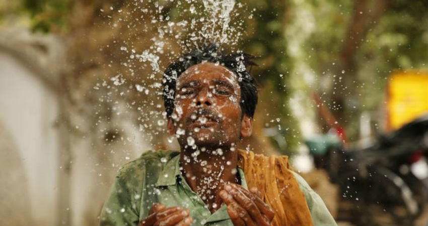
This year, India reeled under a prolonged spell of heat wave with a total of 32 consecutive days. A similar record was set in the year 1988, when heat wave prevailed over the Indian mainland for a total of 33 days at a stretch after 3 consecutive years of droughts in 1985, 1986 and 1987. Extreme heat was also observed in the year 2015, which turned out to be a drought year.
This year, the state of Bihar has already witnessed many deaths related to heat wave conditions. The current year is turning out to be extremely hot for many places. On June 15, Gaya in Bihar recorded 45.6°C as the day temperature, which was 8 degrees above normal. On the same day, Patna also saw the maximum soar to 45.8°C. While the national capital Delhi broke all records with Safdurjung Observatory recording a whopping 48°C. The maximums in stations like Churu, Phalodi and Ganganagar also exceeded the 50 degrees Celcius mark multiple times.
This has been a rather drier June in the country. Only Cyclone Vayu has led to a few rains over some regions. Even the national capital of Delhi observed a 20 day long stretch (from May 26 to June 15) of 40-plus temperatures, which is very unusual for the city. Chandrapur in Maharashtra also witnessed 45-plus temperatures for at least 30 days on a stretch, barring a few days (when temperatures were still above 40-degrees). Phalodi in Rajasthan observed 40-above temperatures for almost 40 days. Severe heat wave conditions are prevailing over Jaisalmer and Phalodi which haven’t observed any rains in the last 3 weeks now. Severe heat wave is going on over Banda of Uttar Pradesh as well which soared above 49°C on multiple days.
Heat Wave Timeline
The southern parts of the country like Telangana, North Interior Karnataka and Marathwada are usually the first to experience heat. Here, peaking temperatures set in as early as the end of March.
This is then followed by Central India, East and then North India which starts experiencing heat by the second half of April.
Telangana, North Interior Karnataka, Gujarat, Odisha, Madhya Pradesh, Bihar, Chhattisgarh, West Bengal, Punjab, Haryana, Delhi and Uttar Pradesh comprise of the most heat wave prone pockets in the country.
On the other hand, Coastal India, Northeast India and hills are mostly spared from extreme heat.
The reason behind Heat Wave
Whenever there is any heat build-up over an area in the pre-Monsoon season of March, April and May, it is succeeded by some thunderstorm activity, which normalizes the temperatures. But, when the pre-Monsoon rains are absent from an area, for days together, heat build-up takes place.
Also, as soon as the Monsoon mitigation takes place in the form of rains starting from South India and then reaching above North, the rising temperatures get arrested.
And this is exactly how the weather has mostly panned out in the country so far.
Relief from the heat
Heat wave has already abated states like Gujarat, Rajasthan, Haryana and Punjab because of the ongoing weather activities there.
Bihar and its adjoining areas are also experiencing some weather activities now. Some more rain and thundershowers are being expected in Bihar in view of the changing weather. Also, a changed wind profile will lead to more rains in the area in the next two to three days. A weather system is also building up in the Bay of Bengal.
Monsoon usually makes an appearance in Bihar on June 10. It’s already been running quite late till now and may make an appearance in the next week or so.
In a country rife with corruption and unease, Zuzana Caputova steps forward as the fresh-faced first female president, sworn in on 15 June, 2019
Zuzana Caputova had been battling to close a toxic landfill in her hometown, Pezinok, in Slovakia for years when she learned that the wife of her closest colleague had been stricken with an aggressive form of cancer. That same week, her godfather was told that he, too, had cancer. “Part of my personal motivation to get involved in this case is that I was scared of cancer,” she says. “And suddenly, in this week, the first week of June 2006, these two roles – the personal and professional – came together.”
That experience convinced Caputova that what counted most was doing her best to win the case and not to worry about the result, which she could not control. She did eventually win it before the European Court of Justice in 2013, and says she now plans to bring that same attitude to her new job.
On 31 March, Caputova, then a 45-year-old lawyer and political neophyte who had never held state office, became the first woman sworn in as president of Slovakia.
At her swearing-in ceremony in Bratislava, the capital, she vowed to continue to work for the forgotten and the dispossessed. “I offer my expertise, emotion and activism. I offer my mind, my heart and my hands,” she said. “I want to be the voice of those who are not heard.” Caputova rode a wave of public disgust with a political system rife with corruption to a victory widely seen as a rebuke of the illiberal and nativist strain of populism that has swept the European continent in recent years.
“I am happy not just for the result, but mainly that it is possible not to succumb to populism, to tell the truth, to raise interest without an aggressive vocabulary,” she told her supporters during her March victory speech.
Caputova is proudly European, supports minority rights and does not shy away from controversial stances, like her support for gay rights, including the adoption of children by same-sex couples. Significantly, she was able to do so in a way that many in this still deeply conservative country did not find threatening, perhaps offering a model for others.
“When I talked about these things, for me, this attitude is based on a value that I believe to be very conservative and Christian – empathy and respect for other people,” she says. “And, for me, this value leads to tolerance and respect.” By any measure, it has been a remarkable year in this small central European nation, which emerged from communist rule in 1989 and became independent in 1993, after a peaceful split with the Czech Republic.
The revolt against the governing party, Smer-SD, began after the murders of a young investigative reporter, Jan Kuciak, and his fiancee, Martina Kusnirova, in February 2018. Kuciak had been looking into the nexus between politicians and the Italian mob, the ’Ndrangheta. A prominent businessman, Marian Kocner, would later be charged with ordering his killing.
But that came only after hundreds of thousands of people filled the streets and town squares across the country, the largest protests since the 1989 Velvet Revolution. The protests brought down the government of the prime minister, Robert Fico, and paved the way for Caputova’s election a year later. But her ascension promises to be anything but smooth, as she is about to enter a political maelstrom that will test her skills and determination.
Fico’s Smer-SD party remains the dominant political force in the country, and the anger at the government that led many voters to embrace Caputova’s reformist vision has also emboldened the country’s far right, with avowed neo-Nazis winning seats in Slovakia’s parliament.
An unlikely supporter of Caputova is Ivan Kocner, the brother of the businessman charged with ordering Kuciak’s murder. His brother also had a stake in the landfill that Caputova fought to close and had once, not so subtly, threatened her. “I remember the first time we met, and her eyes grew wide,” Ivan Kocner, 48, recalls. “She knew I was Marian Kocner’s brother, and she did not have good experiences with the Kocners.”
Here is this group of angry men, very emotional. And she took it all in calmly, got to the essence and then focused on what needed to be done to fix the problem.
By that time, around 2009, Caputova had won a reputation for helping people take on the authorities. Ivan Kocner had gone to her because the mayor of his small village was trying to sell public land to a political patron and he, along with others from the village, wanted it stopped. “Here is this group of angry men, very emotional,” he recalls. “And she took it all in calmly, got to the essence and then focused on what needed to be done to fix the problem.”
They prevailed. “She is not easily influenced or distracted by outside things,” he says. “It is going to take real effort to keep this part of herself.”
While Ivan Kocner became a documentary filmmaker, his brother surrounded himself with people who saw the country’s transition to democracy as a chance to get rich quick. Many of them would go on to become central figures in the organised crime world. Caputova, who was born in 1973, grew up thinking that communist rule could never last. “I remember how schizophrenic it felt,” she recalls. “To be talking with your friends honestly one moment and then having to hide your opinions with other groups.”
Then it all changed. Able for the first time to travel without a permit, her family visited Vienna during the Christmas season in 1989. “I can still remember the dazzling lights,” she says. When she entered college, she intended to study psychology. But she forgot to bring her paperwork and was rejected from the department. So she took up law instead.
While still in school, she worked as a legal assistant in the mayor’s office in Pezinok. “We had a feeling that we needed to care for something else than just ourselves and our studies,” she says. She volunteered to work with local children who had been neglected and abused. She left the mayor’s office in 1998, along with the heads of several other departments, after a disagreement with the administration.
Jaroslav Pavlovic, who has known her since she was a child, would go on to work with her at city hall and, later, joined in the landfill fight, says he remembers her being fired with “the injustice of it all”.
“It was just brutal how the state could ignore the will of the people,” Pavlovic says.
Caputova says she was pregnant when she joined the landfill case. “Motherhood inspired me to get involved,” she says. The case soon took over her life. The day she went into labour, she says, she was completing a legal brief. Pavlovic says she was nothing if not tough and stubborn. There were many times before they won the landfill case that it all seemed overwhelming and hopeless. “She was the one who would motivate others,” he says. “And she took a lot of the burden on herself.”
Slovak president Zuzana Caputova
Pavlovic says she helped him deal with the pressure by introducing him to meditation, something she had been doing for some time to deal with stress. “I try to meditate every day,” Caputova says. She first came across books on Zen meditation as a teenager and has been a regular practitioner for 13 years. “I’m not sure how we’re going to manage that now,” she adds. “But the regular practice is important for me.”
Pavlovic recalls that Caputova first broached the idea of running for president right after a meditation session early last year. “She asked me what I thought,” he says. “I remember she was very unsure about joining politics. My first reaction was, of course, ‘That’s fantastic,’” he says. “But she told me to think about it.”
After thinking it over, he sent her a passage from a favorite book, about how there are two roads one can choose. The dragon’s path, flying up into heaven; and the worm, digging deep into the ground. To do the job of president well, he says, she would have to make the harder choice – to be the worm.
“But on election night,” he says, “I told her that she had finally managed to connect these two roads into one.”
Forty-five-year-old Qasim being dragged in the presence of policemen after a violent mob attacked him. Credit: Twitter
Washington: Mob attacks by violent extremist Hindu groups against minority communities, particularly Muslims, continued in India in 2018, amid rumours that victims had traded or killed cows for beef, an official US report said on Friday.
The state department, in its annual 2019 International Religious Freedom Report, also alleged that senior officials of the ruling BJP made inflammatory speeches against minority communities.
The report says though India’s Constitution guarantees the right to religious freedom, “this history of religious freedom has come under attack in recent years with the growth of exclusionary extremist narratives”.
The report praised India’s “independent judiciary” for often providing essential protections to religious minority communities through its jurisprudence.
The “exclusionary extremist narratives”, the report says, includes “the government’s allowance and encouragement of mob violence against religious minorities”. The “campaign of violence” says involves intimidation, and harassment against non-Hindu and lower-caste Hindu minorities.
“Mob attacks by violent extremist Hindu groups against minority communities, especially Muslims, continued throughout the year amid rumours that victims had traded or killed cows for beef,” it said.
According to some NGOs, the authorities often protected perpetrators from prosecution, it said.
The report said that as of November, there were 18 such attacks, and eight people killed during the year.
On June 22, two Uttar Pradesh police officers were charged with culpable homicide after a Muslim cattle trader died of injuries sustained while being questioned in police custody, the report said.
Mandated by the Congress, the state department in its voluminous report gives its assessment of the status of religious freedom in almost all the countries and territories of the world.
Releasing the report at the Foggy Bottom headquarters of the state department, secretary of state Mike Pompeo said the report was like a report card which tracks countries to see how well they have respected this fundamental human right.
Government’s failure to act
In the India section, the state department said that there were reports by non-governmental organisations that the government sometimes failed to act on mob attacks on religious minorities, marginalised communities and critics of the government.
The state department said that the Central and state governments and members of political parties took steps that affected Muslim practices and institutions.
The government continued its challenge in the Supreme Court to the minority status of Muslim educational institutions, which affords them independence in hiring and curriculum decisions, it said.
“Proposals to rename Indian cities with Muslim provenance continued, most notably the renaming of Allahabad to Prayagraj. Activists said these proposals were designed to erase Muslim contributions to Indian history and had led to increased communal tensions,” the state department said.
There were reports of religiously motivated killings, assaults, riots, discrimination, vandalism and actions restricting the right of individuals to practice their religious beliefs and proselytise, the annual report said.
However, noting the positive developments, the report says some government entities made efforts to counter increasing intolerance in the country. Citing Rajanth Singh, previously the home minister, it said there was a 12% decline in communal violence compared to the previous year.
Senior US government officials underscored the importance of respecting religious freedom and promoting tolerance throughout the year with the ruling and opposition parties, civil society and religious freedom activists, and religious leaders belonging to various faith communities, the report said.
India has 1.3 billion population as per July 2018 estimate.
According to the 2011 national census, the most recent year for which disaggregated figures are available, Hindus constitute 79.8% of the population, Muslims 14.2%, Christians 2.3% and Sikhs 1.7%.
Groups that together constitute less than one per cent of the population include Buddhists, Jains, Zoroastrians (Parsis), Jews, and Baha’is.
Suggestions to the US government
The document makes recommendations to the US government to improve religious freedom in India. It says the US should press India to allow a USCIRF delegation to visit the country and evaluate the conditions for freedom of religion.
The report says since 2001, USCIRF has attempted to visit India in order to assess religious freedom on the ground. “However, on three different occasions—in 2001, 2009, and 2016—the government of India refused to grant visas for a USCIRF delegation despite requests being supported by the State Department,” it says.
The US government could work with India to “create a multiyear strategy to ebb the flow of hate crimes targeting religious minorities”, the report says. It suggests measures such as pressing state governments to prosecute religious leaders, government officials and media personalities who incite violence against religious minority groups through public speeches or articles.
The US should encourage India to pass the Protection of Human Rights (Amendment) Bill, 2018 to establish national and state human rights commissions and human rights courts, the report says.
It also asked the US government to ensure that India’s Central government does not use the Foreign Contribution Regulation Act (FCRA) to “target international missionary and human rights groups”.
The CBI recently registered a case against the Lawyers Collective, a NGO run by prominent advocates Indira Jaising and Anand Grover, for alleged misuse of the FCRA. The NGO denies these allegations and said its office bearers were “personally being targeted for speaking up in defence of human rights, secularism and independence of the judiciary in all fora”.
(With PTI inputs)
Forty-five-year-old Qasim being dragged in the presence of policemen after a violent mob attacked him. Credit: Twitter